Understanding Word Embeddings (Word2Vec)
From Count-based methods to Distributed Word Embeddings: The Evolution of NLP Representations

Preview
In the mid-1950s, an experiment was conducted in collaboration between Georgetown University and IBM. The objective of the experiment was to use a computer to translate 60 sentences from Russian to English. Although the results were inaccurate, this experiment marked a significant milestone in developing NLP and machine translation. We’ve come very far since this advent. Thanks to our progress in NLP, machines have become so adept at understanding the human language that they can even detect sarcasm, which is still a toil for some humans.
Before extensive use of linear algebra and neural networks to represent words, ML practitioners used count based methods like (i) Bag-of-words (BoW) and (ii) Term frequency-inverse document frequency (TF-IDF) to do the same. Let’s get a brief overview of these two methods before we understand a much more advanced way of representation.
Bag-of-words (BoW): A method that counts the frequency of words in a corpus and assigns that number to it. A vector is formed for each sentence or document in the corpus, where each element represents the frequency of a particular word in that sentence or document.
The problem with this approach is it does not consider the order in which words appear. No context.
This also does not consider the semantics of the word. Similar words should have similar numerical representations.
Also, it causes a lot of sparsity1. If you notice, many values in the array are zero. Imagine if we have a large corpus, a waste of computational resources.

The Bag-of-Words Model: A clever trick for fooling machines into understanding language Term Frequency Inverse-Document Frequency (TF-IDF): TF-IDF calculates the most important words in the corpus. It reduces the importance of common words and gives more weight to rare, informative words. Consider it to be a weighting scheme for information retrieval. For example, if I analyze annual reports of Airbus, words like “sky,” “aircraft,” etc. might be used often but are unimportant, so I’d down-weight those words. TF-IDF does precisely that.
Even TF-IDF, like BoW, gives no importance to the semantics of the language.
There’s a chance rare words might be given too much importance because the inverse document frequency value may be too high.
It lacks context; therefore, it cannot capture deeper relationships in a language.


Word2Vec
Assume we take all the words in the corpus and project them onto an n-dimensional vector space where each word gets assigned a vector, and considering two or more words appear together in the corpus consistently, the vector representations of these words shall also be closer in the n-dimensional space that we create. Therefore, when we try to calculate the distance between both word vectors, it should be minimal. This is a high-level overview of what word2vec tries to do. So how does word2vec achieve this?
Skip-Gram & CBOW (Continuous Bag of Words)
These are two popular architectures to train the word2vec neural network to get word representations. If we take the sentence “I love eating pizza 🍕” the CBOW method could guess that the term “pizza” is most likely to appear based on the nearby words “I love eating.” On the other hand, the Skip-gram method might guess that the words “I” and “love” are likely based on the context of the word “pizza” because, let’s face it, who doesn’t enjoy pizza? Therefore CBOW tries to predict the target word given the context words, and Skip-gram tries to predict the context words given the target word.
The decision to choose between the two depends on the size of the available dataset and the complexity of the context in the text. A good note is that CBOW works well on small datasets where predicting the target word based on the context is relatively simple. Skip-Gram is the choice to pick when the dataset is more extensive, and predicting the context of the target word is a complex task. Also, CBOW takes less training time to converge the global minima2 as it predicts the target word from the sum of all context words.
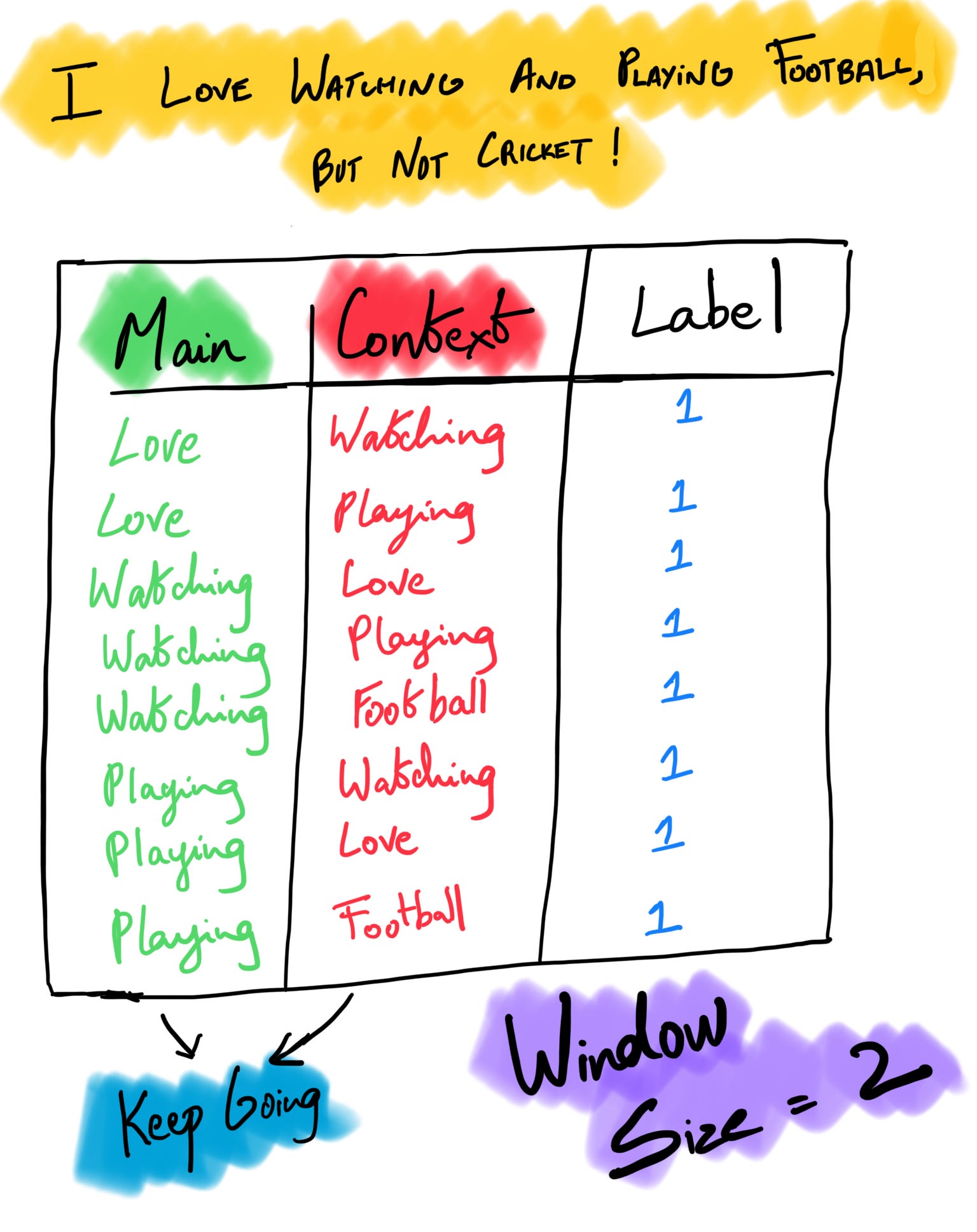
For the purposes of this article, let’s go ahead with skip-gram. The below image shows the main & context words with a window size of 2. A window size of 2 means two words before and two words after the target word. Stopwords are generally removed from the text as a preprocessing step; hence you do not see the words “I” & “and” in the image. This process is insufficient to feed into the model because we have only considered words that occur together and not words that do not. In the next step, we must ensure our potential neural network learns both instances to map what words appear together and what do not.
Negative Sampling
Instead of just considering words that occur together, this step builds scenarios where they do not. For example, in the above image, the words “love” & “cricket” do not occur together; therefore, it would get a label score of 0 which would then be added to the above table. Adding this layer to the process would give us a more holistic view of the corpus than a biased one because we’re leveling the field. Rather than updating the neural network weights for each training example, negative sampling selects a few “negative” examples at random to update the weights.
Prediction
How to turn your words into vectors?
Initialization: The main and context vectors are initialized randomly with small values between -0.5 and 0.5. The main vector represents the predicted target word, while the context vector represents the words in its context (if it’s a neighborhood word, how shall we represent it?). If we have a vocabulary size of 10,000 and a vector dimensionality of 300, each main and context vector will have 300 random values between -0.5 to 0.5.
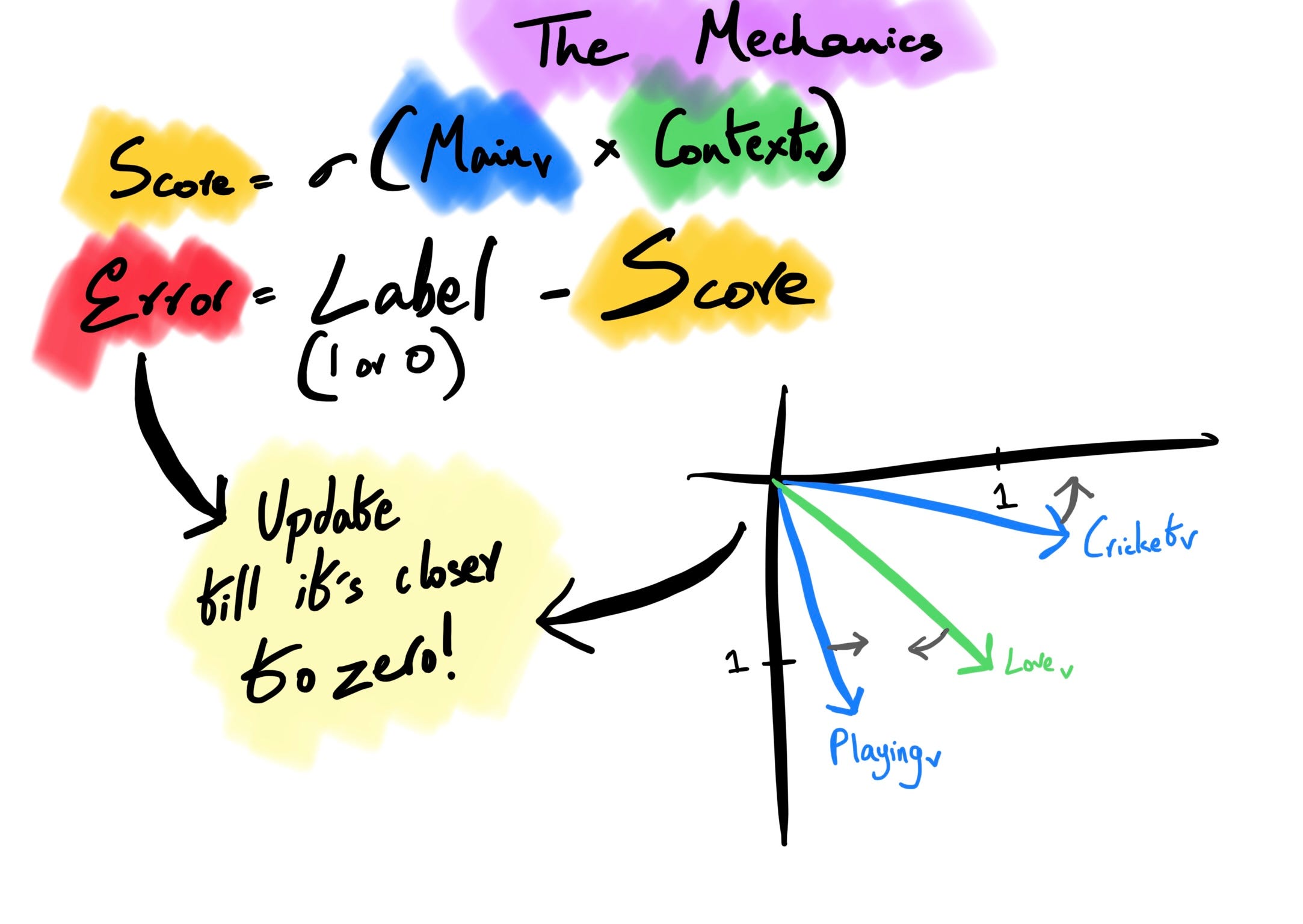
Computing Score: For every main vector and context vector, we compute a score by multiplying both the matrices to a result. The dot product is run through the sigmoid function (σ)3 to get a value between 0 and 1. A large product put into a sigmoid function gives something closer to 1, meaning the two-word vectors are closer in the n-dimensional space. Since we initialized these values randomly, the error rate would be significantly high; the next step is where we optimize this using a loss function.
Backpropagation: The error (difference between predicted score and actual labels) is calculated and propagated backward through the neural network to adjust the weights to get an iterated lower error score. During training, the main and context vectors are updated to improve the model’s ability to predict the surrounding context of a word. This process continues until the model converges to an optimal set of main and context word vectors.

The network trains to bring “love” and “playing” close together and push cricket away. “Update” here means backpropagating to reduce the errors. We can build semantic and syntactic relationships between words by performing this delicate vector dance in an n-dimensional space. This helps us with NLP tasks such as text classification, information retrieval, and machine translation. The above example only takes a window size of 2 words, but more complex relationships can be built with broader window sizes.