
Principal Component Analysis
A fascinating intersection of algebra and statistics to reduce complexity

PCA, short for Principle Component Analysis, is one of the core concepts for dealing with high-dimensional data. A few examples of high dimensional data could be a sensor collecting data across 100 different attributes every x minutes, financial data of a company across multiple metrics/financial ratios from its annual financial reports, or images where each pixel acts like an independent feature. High-resolution photos translate into high dimensional data (this means high storage requirements too). Therefore, we can now agree that performing data analysis and predictive modeling on this would incur a higher computation cost. This is where PCA can be used to reduce the data's dimensionality to ensure model training is quicker and more efficient. Think of what we're about to delve into as extracting the most essential features that have the maximum impact on whatever we're trying to predict instead of keeping everything in our toolbox.

PCA Math
This article aims to walk you through the math behind the PCA so we understand what’s happening behind the scenes when we instantiate PCA from sklearn.decomposition1 in our Python scripts. There are broadly five steps, from ingesting raw data to extracting the transformed data’s principal components. Ultimately, the math we walk through is compared against the sklearn output to check for consistency. The takeaway here is understanding data transformation through PCA at a granular level. Let’s dive in.
1. Data Centering
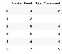
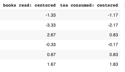
The first step is to standardize our data. This translates into our data having a mean of 0 and a standard deviation of 1. This brings our data of different units to the same scale2. We do this by subtracting the mean from individual observations in the column. The arithmetic mean of “books read” comes to 5.33, whereas “tea consumed” comes to 3.16. Therefore we subtract this value from each respective observation. Eg; 4 - 5.33 = -1.33
2. Calculating Covariance Matrix
variance = (1/(n - 1)) * Σ[(xi - mean)²]Let’s take this step by step. First up is variance, a measure of the dispersion of a dataset; it is the average of the squared differences from the mean. If you’ve noticed the above formula for calculating variance, we’ve already performed xi minus the mean. The remaining step is to sum the squared values of each column and divide it by the number of observations minus 1. For example, to calculate the variance of “books read” (already centered):
((-1.33)^2 + (-3.33)^2 + (2.67)^2 + (-0.33)^2 + (0.67)^2 + (1.67)^2 / 5The above is repeated to find the variance for “tea consumed.” Now that we have individual variances, we find the covariance, which measures how much two variables change together3. To find this value for our data, we multiply the values of our centered data:
((-1.33) * (-1.17) + (-3.33) * (-2.17) + ...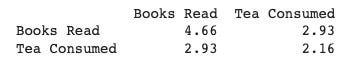
3. Computing Eigenvalues & Eigenvectors
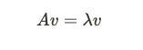
An eigenvector v is basically a non-zero vector that satisfies the above equation. If you multiply square matrix A by a column vector v and get a vector that is a number (lambda) times the old vector, the vector v is called the eigenvector matrix A. We can think of this as multiplying matrix A (covariance matrix) by vector v; The new vector does not change direction after the transformation. The new vector should have the same direction as the original vector. Simply put, if the A*V is (9,3) and if V here is (3,1), then we can say V is an eigenvector of A because it has linearly increased in size without changing the direction (3*3 & 1*3). Sweet, now let’s come to eigenvalues.
Given a square matrix A, an eigenvalue λ is a scalar value that satisfies the below equation. The eigenvalue tells us how much the eigenvector changes in size when multiplied by the matrix. For the above eigenvector example, the vector was thrice as long (9,3) as the original vector (3,1); therefore, the associated eigenvalue is 3.
The eigenvectors of the covariance matrix represent the directions along which the data varies the most. The corresponding eigenvalues represent the amount of variance of the data along each of these directions. By choosing the eigenvectors with the largest eigenvalues, we can capture the most important patterns in the data and project the data onto a lower-dimensional space that retains most of its variation.
i) Computing Eigenvalues

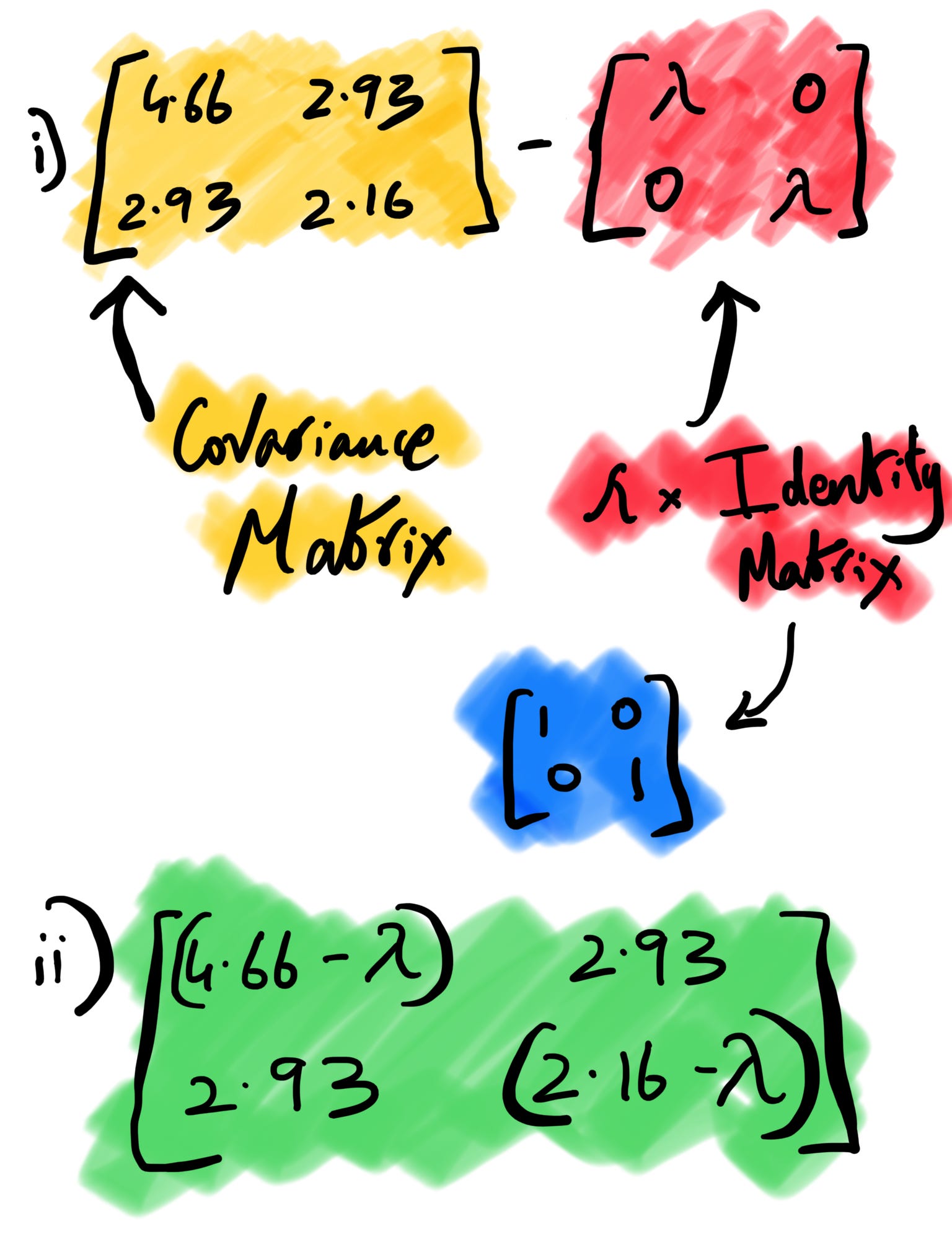
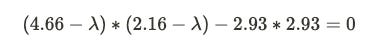
Let’s understand the above formula. The I here is identity matrix4 , det is the determinant of matrix5 and A is the covariance matrix we computed earlier. We subtract our covariance matrix from the λ * identity matrix. After subtraction, we take the determinant of the matrix, which is nothing but the product of the first diagonal minus the product of the second diagonal in a 2*2 matrix.
ii) Computing Eigenvectors
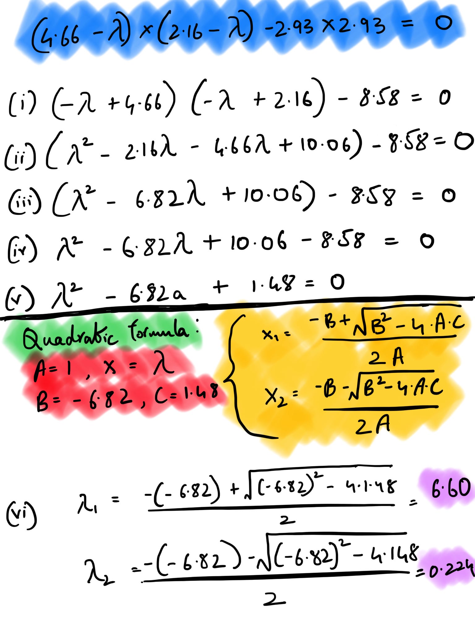
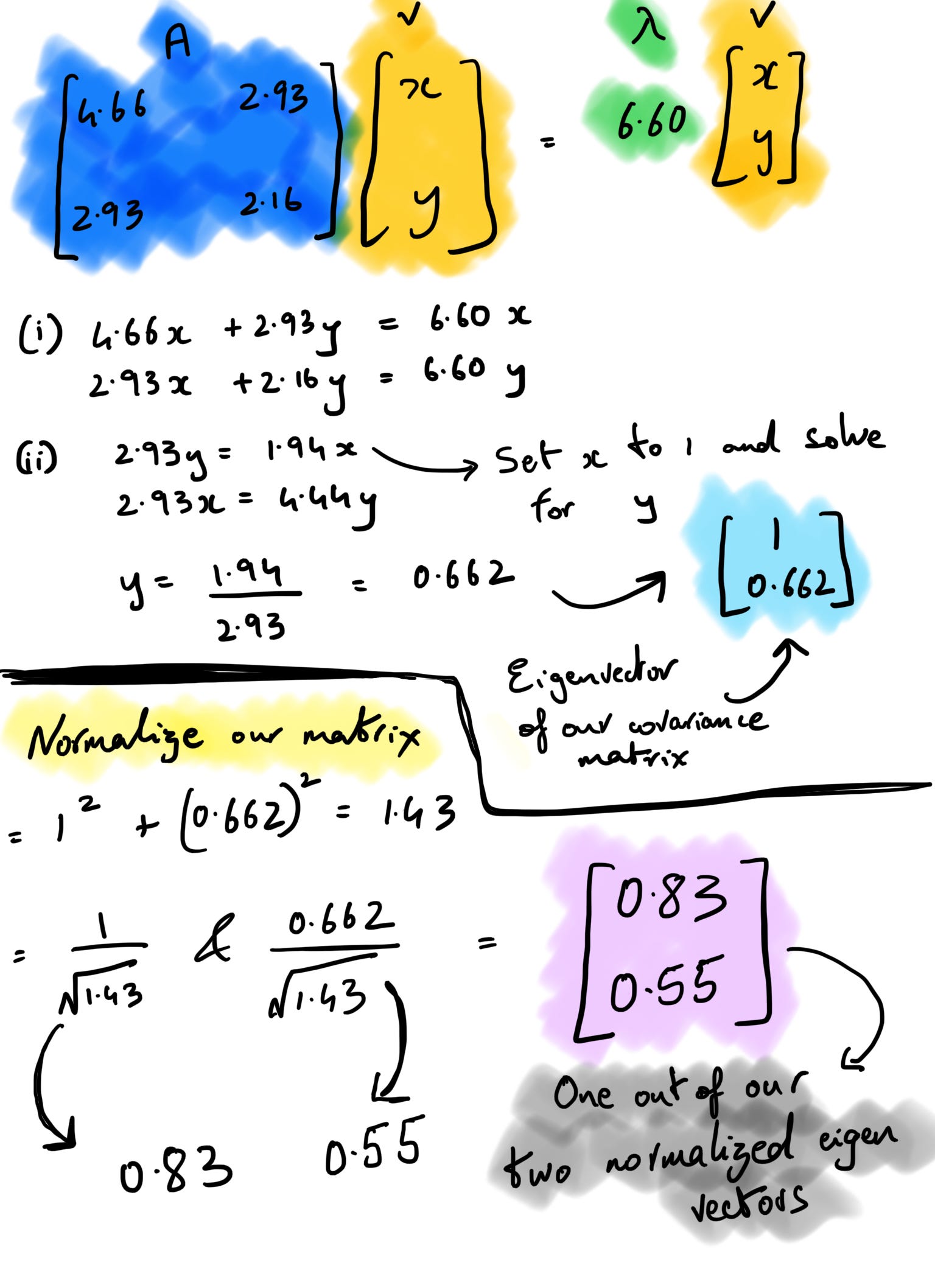
So far, we’ve just ensured the equation holds with the lambda values we’ve derived. Now let’s calculate the corresponding eigenvectors for these two eigenvalues. The eigenvector equation states that the result of our covariance matrix * vector v should equal one of our eigenvalues * the same vector v.
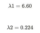
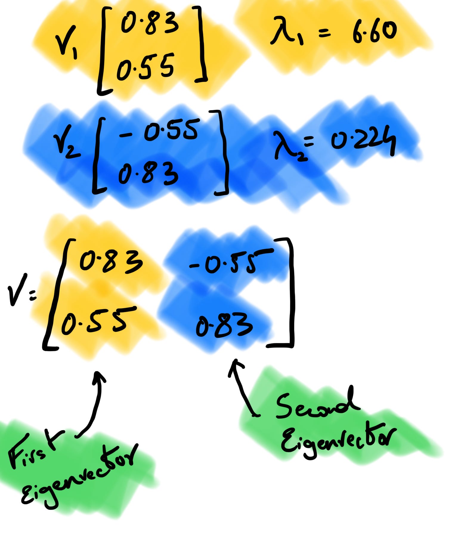
If we assume v to be (x, y), A to be our covariance matrix, and λ to be 6.60 and solve for it using the linear system of equations, v turns out to be (0.83, 0.55) after normalization. In the snapshot below, the (i) is to perform matrix multiplication before we find out the y value by substituting x as 1 (you can do the opposite too). If we perform the same set of operations setting λ = 0.224 as we get our second set of eigenvectors as (-0.55,0.83).
4. Order the Eigenvectors
We order our eigenvectors by the largest corresponding eigenvalues. We concatenate the two eigenvectors into one matrix and use this matrix to calculate our principal components. When performing PCA, the eigenvectors of the covariance matrix are used to determine the principal components of the data, and the eigenvalues are used to rank the importance of these components. The principal components with the largest eigenvalues capture the most variation in the data and are, therefore, the most important.
5. Calculate Principal Components
The final step is to simply take our final matrix v and multiply it against our centered data to find our principle components. If you compare the two outputs, the results are mirror opposite in terms of arithmetic signs, this could be because of how different statistical tools project the data. But, the important thing to take away is that we if we compute the explained variance our PC1, it comes to 0.96, the same as sklearn output therefore the sign of the eigenvectors and eigenvalues does not affect the results of principal component analysis, as long as the signs are consistent within a given analysis6.
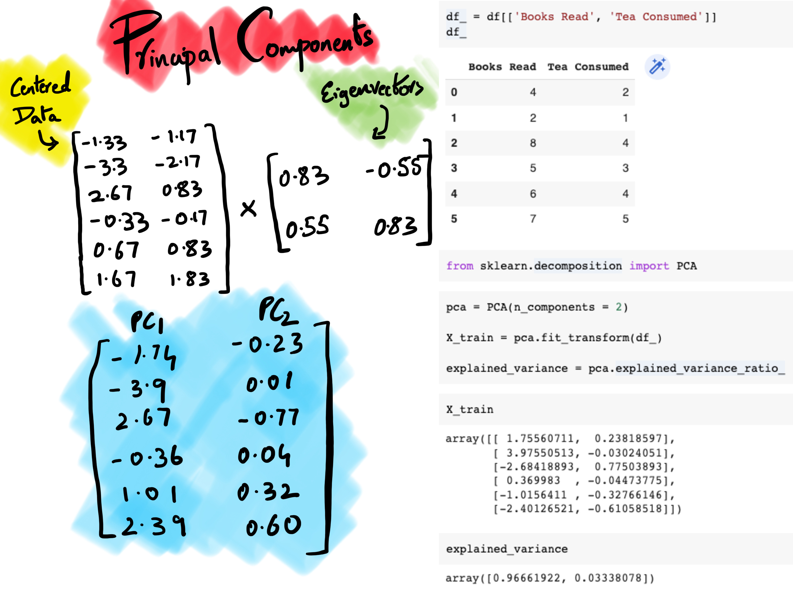
Since, we’ve established PC1 captures 96.6% of variance we can afford to remove PC2 from our analysis and build our potential ML model on just PC1. One way to decide how many principal components to consider is to understand how much loss of variability are we willing to sacrifice. For example, if PCA is applied on 100 features and the first 7 principal components explain 95% of variability in data, that’s a pretty good case to consider since it would reduce the computation requirements significantly in exchange for minor loss of data.
Conclusion
The math we performed happens at a significantly larger scale when dealing with big data, and modern Python libraries’ ability to churn out these figures with a couple of lines of code is impressive. Ideally, PCA should be used when there are many variables and/or when the variables are highly correlated. It can also be used when the goal is to identify the essential variables or to reduce the dimensionality of the data for easier visualization or interpretation. It’s an effective technique that improves performance, reduces data redundancy/noise, and allows for data compression as we store only the reduced dimensions.
Height and Weight: Height is measured in centimeters or inches, while weight is measured in kilograms or pounds. These variables have different units of measurement and scales, so they would need to be standardized for algorithms to compare them.
A positive covariance indicates that the two variables tend to increase or decrease together, while a negative covariance indicates that they tend to have opposite behaviors. A covariance of zero indicates that there is no linear association between the variables.
There are small differences between our manually calculated numbers and sklearn, primarily due to how Python stores numbers (float62 or float32) which is more precise.